Introduction
One of the most popular techniques for classification is the binary classification method. It’s simplicity, interpretability, and scalability are big advantages. Although more recent methods for classification have gotten a fair amount of attention the logistic regression stays a strong contender for many problems.
I wrote this article because of a training I gave on the subject for some junior data scientists. Although I had worked with it before, I never took the time to understand some of it’s “finer” points. Coming from a mathematics background, I like to understand how things work and why they work. I feel this helps in understanding what the strengths and weaknesses of something are, and how it’s connected to similar mathematical machinery. For those of you who are interested, here are some of the things I discovered.
To keep things simple we’ll be limiting ourselves to the two (e.g. 0 and 1) class problem.
Relation between thresholds and decision boundaries
Most of you probably know that in order to get the binary output we want, we must choose a threshold value. Probabilities below this threshold are set to 0, and above it are set to 1. Visually we can think of it this way:
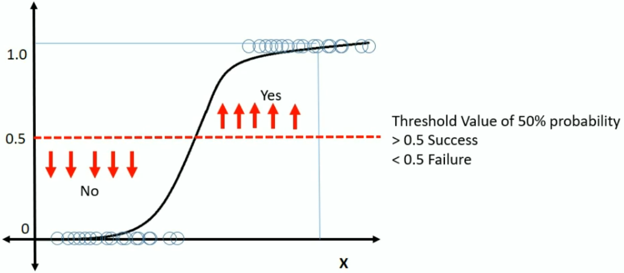
You might wonder, how does that relate to a decision boundary? The decision boundary refers to the hypersurface that splits the feature space into the two output classes. Which side of the boundary a point is determines how it gets classified by the model.
Given a probability threshold, it’s pretty easy to find this boundary with a little linear algebra. Let’s take $t = 1/2$ and see what what the boundary is:
\[\begin{align} P(Y = 1 | X = x) & = \frac{1}{1 + e^{\beta^\intercal x}} = 1/2 \end{align}\]We can rewrite this as
\[\begin{align}\frac{1}{1 + e^{\beta^\intercal x}} & = \frac{1}{2} \\ 1 + e^{\beta^\intercal x} & = 2 \\ e^{\beta^\intercal x} & = 1 \\ \beta^\intercal x & = 0\end{align}\]So there it is, our boundary for $t=0.5$ is the line $\{x \in \mathbb{R}^n: \beta^{\intercal}x = 0 \}$, which is a hyperplane in $\mathbb{R}^n$. If we include nonlinear functions of our features as additional features, this will add nonlinearities to this decision boundary.
Deriving Cross-Entropy from Maximum Likelihood
So now that we’ve defined the model, we also need a function which tells us how well the model fits the data we’re training on. There are lots of loss functions to choose from, so why is the cross-entropy usually taken for logistic regression?
The short answer is it’s equivalent to the Maximum Likelihood Estimator here, which has all kinds of nice properties. It’s pretty easy to derive the cross-entropy from the MLE, so we’ll show that here. Lets start with the expression of our trustworthy log-likelihood:
\[\begin{align} \log \mathcal{L}(\beta) & = \sum_{i=1}^n\log P_\beta(Y = y_i|X=x_i) \\ & = \sum_{i=1}^n\log P_\beta(Y = 1|X=x_i)^{y_i} + \log P_\beta(Y = 0|X=x_i)^{(1 - y_i)} \\ & = \sum_{i=1}^n y_i\log \hat{y}_\beta(x_i) + (1 - y_i)\log (1 - \hat{y}_\beta(x_i)) \end{align}\]which is exactly the cross-entropy loss.
Geometric Interpretation of L1/L2 Regularization
L1/L2 regularization (also known as Ridge/Lasso) is a widely used technique for reducing model overfitting. We restrict the size of the model’s weights, which restricts how complex the model can become. This increases bias, reduces variance, and allows for better generalization on the test set.
In order to regularize our problem, we minimize the original problem:
\[\sum_{i=1}^n L(\beta, x_i) = \sum_{i=1}^n y_i\log \hat{y}_\beta(x) + (1 - y_i)\log (1 - \hat{y}_\beta(x_i))\]but we add a restriction, namely:
\[\text{arg}\,\text{min}_\beta\sum_{i=1}^n L(\beta, x_i), \quad \text{such that}\, \|\beta\| \lt C\]for some $C > 0$ which determines how strong we want to regularize. If we use the L2-norm for $\Vert\beta\Vert$ we get Ridge regularization, and with the L1-norm we get Lasso. Smaller values for $C$ correspond with stronger regularization.
Feature Selection with L1/L2 regularization
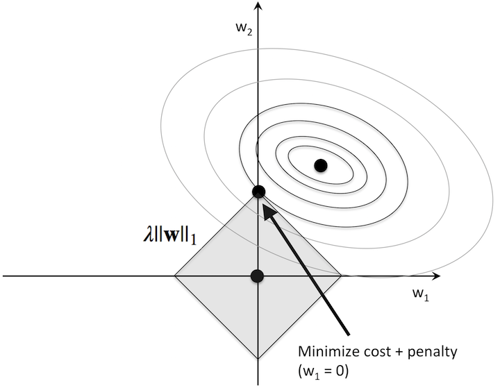
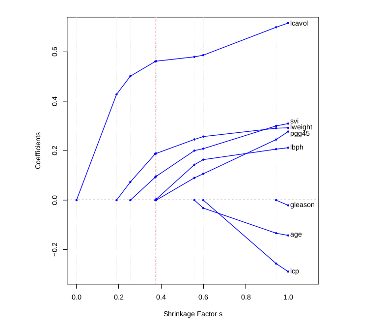
A key difference between the two kinds of regularization is that lasso “turns-off” features, while ridge only reduces their values. Why this happens has a nice geometric explanation which I took from Elements of Statistical Learning.
Ridge
It can be shown for logistic regression with cross-entropy loss that the loss function is convex, with elliptical level sets. The gives the optimization problem shown below when $\beta = (w_1, w_2)$:
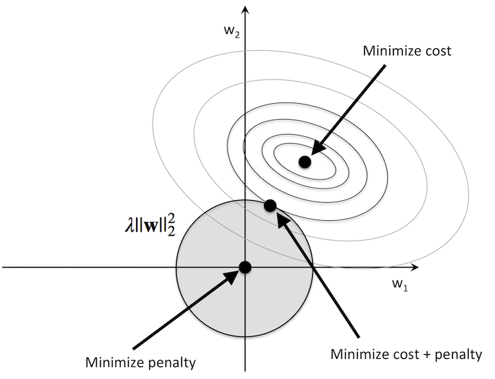
In this picture, you can see that if we’re using the L2-norm, the unit-ball takes the form of a circle. This means that the minimum will be where the black dot is, and this will usually be at a point where $w_1, w_2 > 0$, and as we wanted both fitted weights are smaller than the original one.
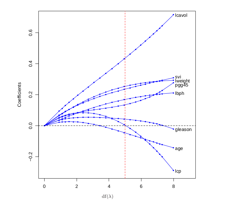
To see this happening with a real model, take a look at this graph which plots the value of various weights as we increase the amount of regularization by reducing $\text{df}(\lambda)$.
Lasso
Things work a little differently for Lasso regularization with the L1-norm. In this case the unit ball looks like a diamond, which causes the constrained minimum to more often fall on the corners of the diamond. These corners correspond with features being set to zero.
It’s a bit harder to visualize this picture in higher dimensions, but just like the ridge regression we can plot the weight values against the regularization strength to visualize this “turning-off” of features.
Lagrange Duals and Regularization
The last thing I want to share is a detail on regularization I saw lot’s of authors skip over. Usually regularization is written as this minimization problem, the one with regularization term added to the loss function
\[\text{arg}\,\text{min}_\beta\left(\sum_{i=1}^n L(\beta, x_i) + \lambda \Vert\beta\Vert\right)\]I wanted to figure out why this was equivalent to
\[\text{arg}\,\text{min}_\beta\sum_{i=1}^n L(\beta, x_i), \quad \text{such that}\, \|\beta\| \lt C.\]The second is essential to the whole geometric interpretation, while the first is the form used for gradient descent, so I wanted to see this equivalence for myself.
After some research, I found out these two formulations are equivalent due the strong Lagrangian principle. For the curious, this comes from the field of convex optimization and tells us which conditions are necessary for these two types of problems to be equivalent. For more information on this duality you can check out this paper which formally proves this result.
