Opening Remarks
Recently at work we had a hackathon on tensorflow, which is something I’d tried (running examples) but never really took the time to play with it. I’d like to share my experiences with the tensorflow computational graph, and some of the flexibility it has to do cool stuff.
I’m not a tensorflow expert, so please let me know if there are any inaccuracies I need to correct
Quick Introduction to Tensorflow
The computation graph
In order to do anything in tensorflow, you need to create a so called computation graph. This is the main construct used to break things down into problems your GPU can efficiently solve. Like Numpy and PySpark, python is just a wrapper for telling other engines to run your computations. In the case of tensorflow, this is for CUDA and your GPU.
Sending data from your GPU to python and back creates a lot of performance overhead, so the computation graph is a way of helping you do that as little as possible.
You define a computation graph using special tensor objects (eg. constants, vectors, matrices) and tensor operations (eg. multiply, weighted sum, apply loss function). Inputs to your graph (like a training dataset) are defined as placeholders.
Calculating a matrix inverse, the hard way
Say we want to make a simple computation graph, but a little more complicated than adding two numbers. Let’s take a square matrix as input, and multiple it by some set matrix $A$. Our goal is to create a graph that finds the matrix inverse $A^{-1}$, which we enforce with the loss. This function tries to make the output as close to the identity matrix as possible.
import tensorflow as tf
import numpy as np

# We'll put this into the graph later
rand_matrix = np.random.randint(0, 10, (10, 10))

# We start making our graph here
x = tf.Variable(np.zeros((10, 10)), dtype=tf.float32, name="A")
A = tf.constant(rand_matrix, dtype=tf.float32)
output = tf.matmul(x, A)
id_mat = tf.constant(np.identity(10), dtype=tf.float32)
loss = tf.reduce_sum(tf.abs(output - id_mat))

# Here we define some "meta-graph" stuff
optimiser = tf.train.AdagradOptimizer(learning_rate=0.01).minimize(loss)
init_op = tf.global_variables_initializer()
So in the above section we defined:
- some variables (stuff which get updated and persists between runs)
- some constants which don’t change
- matrix multiplication, which transforms our input into an output in our case
- a loss function
- an optimiser which changes the variables in the graph to minimize the loss
- a variable initializer, which creates initial states for any variables which are defined using a distribution (we don’t use those)
With this defined, we can start training the model.
# Number of passes over the data
epochs = 100_000

# Context managers work nicely with tensorflow sessions
with tf.Session() as sess:
    sess.run(init_op)
    for e in range(epochs):
        _, epoch_loss = sess.run([optimiser, loss])
        if e % 100 == 0:
            print(epoch_loss)

    # Lets evaluate the learned matrix A
    x_ = sess.run(x)
    print(x_.dot(rand_matrix))
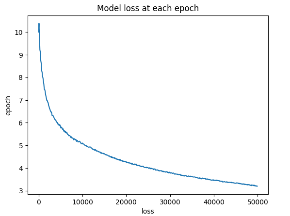
Running the optimizer once will update the variable x by one step. In order to get a good estimate, we run the optimizer 100,000 times. With the last bit of code, we extract the learned matrix x from the tf session and check if it is indeed close to the inverse.
In order to see if the algorithm is converging we can look at the loss of the model vs the training epoch. Just to be sure we also check to see if the learned matrix x actually does approximate $A^{-1}$ (it does).
We trained our first tensorflow model! This little excercise helped me understand the concepts of the computation graph, and it should make the later example easier to follow if you’re new to tensorflow.
Classifying MNIST with tensorflow
Now that we understand the basics of tensorflow, lets build single-layered neural network using tensorflow to classify these images.
Model Definition
We’ll rescale the images to 28x28 pixel images and represent these by a 28x28 matrix, where each matrix entry represents the pixels color-intensity with a number between 0 and 1.
The output of the network will be a one-hot encoding of the numbers 0-9, so each one will be a 10-dimensional vector.
Finally, the network connecting the inputs to the outputs will be a single densely connected layer, a relu activation function, and a softmax to ensure we are left with a probability vector as the output.

Implementation
Just like the previous example, we’re going to define our network in a computation graph, using tensors and tensor operations. We’ll use a placeholder x for our input images and y for the one-hot encoded label. Note that we reshaped the images from a 28x28 matrix to a vector of length 784.
Here’s the graph we used for this:
import tensorflow as tf
from tensorflow.examples.tutorials.mnist import input_data
import numpy as np

# Read data
mnist = input_data.read_data_sets("MNIST_data/", one_hot=True)

# Python optimisation variables
learning_rate = 0.1
epochs = 50
batch_size = 100

# declare the training data placeholders
# input x - for 28 x 28 pixels = 784
x = tf.placeholder(tf.float32, [None, 784])
# now declare the output data placeholder - 10 digits
y = tf.placeholder(tf.float32, [None, 10])

# now declare the weights connecting the input to the hidden layer
W1 = tf.Variable(tf.random_normal([784, 300], stddev=0.03), name='W1')
b1 = tf.Variable(tf.random_normal([300]), name='b1')
W2 = tf.Variable(tf.random_normal([300, 10], stddev=0.03), name='W2')
b2 = tf.Variable(tf.random_normal([10]), name='b2')

# calculate the output of the hidden layer
hidden_out = tf.add(tf.matmul(x, W1), b1)
hidden_out = tf.nn.relu(hidden_out)
y_ = tf.nn.softmax(tf.add(tf.matmul(hidden_out, W2), b2))
y_clipped = tf.clip_by_value(y_, 1e-10, 0.9999999)
cross_entropy = -tf.reduce_mean(tf.reduce_sum(y * tf.log(y_clipped)
                         + (1 - y) * tf.log(1 - y_clipped), axis=1))

# add an optimiser
optimiser = (tf.train.GradientDescentOptimizer(learning_rate=learning_rate)
                .minimize(cross_entropy))

# finally setup the initialisation operator
init_op = tf.global_variables_initializer()

# define an accuracy assessment operation
correct_prediction = tf.equal(tf.argmax(y, 1), tf.argmax(y_, 1))
accuracy = tf.reduce_mean(tf.cast(correct_prediction, tf.float32))

# Training the network
with tf.Session() as sess:
    sess.run(init_op)
    total_batch = int(len(mnist.train.labels) / batch_size)
    for epoch in range(epochs):
        avg_cost = 0
        for i in range(total_batch):
            batch_x, batch_y = mnist.train.next_batch(batch_size=batch_size)
            _, c = sess.run([optimiser, cross_entropy], feed_dict={x: batch_x,
                                                                   y: batch_y})
            avg_cost += c / total_batch
        print("Epoch:", (epoch + 1), "cost =", "{:.3f}".format(avg_cost))
    print(sess.run(accuracy, feed_dict={x: mnist.test.images, y: mnist.test.labels}))
Let’s check out the output of this model, and see if it did what we wanted to. We’ll look at the cross-entropy loss on the training set, test set, and the overall accuracy on the test set, for each epoch.
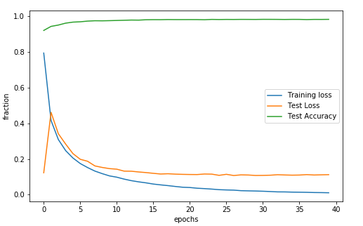
This will learn the network weights $W_1, b_1, W_2, b_2$ and give a pretty decent accuracy for classification, 98% on the test set!
Looking into our network
Image fingerprints
As this was my first time working with tensorflow and a neural network, I was interested in dissecting the network a bit. The input and output layers aren’t too interesting, so I thought I’d look at the hidden layer for out-of-sample images.
Getting each hidden layer was quite simple. If you want the hidden layers for all 0 images:
- Create a tf-session and train the neural network. Don’t close the session!
- Filter the test images to only the 0 ones.
- Running
sess.run(hidden_out, feed_dict={x: input_data})will return a tensor where each row is the hidden layer for the images that you fed it.
If you plot this matrix for each label, we get the following image:
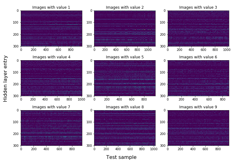
So what do we see here? One thing that is pretty clear, is that each class shows clear horizontal bands across all the test images. Each vertical stripe is the hidden layer vector for that specific test set image. If we see a horizontal stripe, that means that vector entry is “activated” in most of the images with that label.
This unique pattern of bands is what the second bit of linear algebra ($A_2\cdot x + b_2$) uses to classify these images, as the combination is a kind of unique indentifier or fingerprint for each image. Our network learned this itself, which is super cool!
Estimating optimal input images
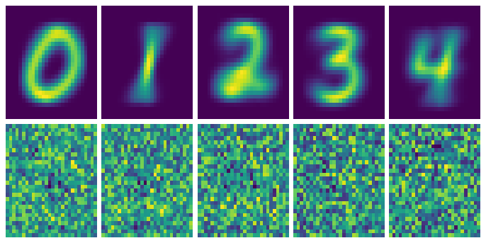
After seeing the patterns in the hidden layers, I was curious what the “otpimal” image would be for each class. The first approach I tried wasn’t very feasible, reversing the network direction to give an input for a specific output. This has to do with the fact that we reduce a $784 \times 1$ vector to a $10 \times 1$ vector, so a lot of information is lost.
There’s another approach we can use, where we train another model which tries to learn the input vector which best outputs one of the outputs corresponding with the one-hot encoded labels. So we try to find the best image input for every output number, according to the network, or technically we’re finding the image vector $\hat{V}_i$ which minimizes the cross-entropy loss between it’s output $\hat{y}_i$ and the unit vector $e_i$ for every $i =0,1,\cdots,9$. The code for this can be found here.
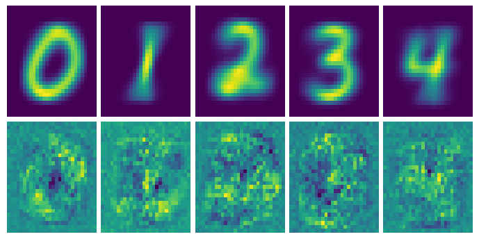
Here are the first images I got with this approach. The images on the top are the average pixel density of all the test sampes, and on the bottom are the “ideal images” according to the neural network.
Regularization to the rescue
So it seems that since our input image has 784 free parameters and we’re trying to create a vector of length 10. Our model is seriously overfitting.
I tried regularization (I wasn’t sure what else to do) and started out with the L1 version. That killed most of the pixels except for a few. L2, on the other hand, was a little more gentle and worked like a charm! Adding a penalty*tf.reduce_sum(x**2) to the cross-entropy term allows us to add a little bias and reduce the variance, giving this much improved version.
L2 regularization with a penalty of 0.25 gave these optimal images
So we finally get some patterns in our ideal images. In each of the images we can roughly make out each of the numbers, but there are some strange irregularities in them.
These irregularities might be the pixels the network finds important for distinguishing numbers, but maybe they’re artifacts from the regularization. Pretty neat though, as there are clearly patterns in the unique areas of each number.
The end
For those of you who held out until the end, here’s a ![]() . I hope you either read something interesting or learned something new along the way.
. I hope you either read something interesting or learned something new along the way.
I’m still new to the whole ML-blogging, so if you’ve got any reactions or tips please leave a message in the comments. You would really help me make the blog better!