This post is the first of a series of posts that serve as an introduction to the field of Machine Learning for those with a mathematical background. They’ve been based off of the Cornell “Machine Learning for Intelligent Systems” course, which has generously put all the classes on youtube. My thanks to Kilian Weinberger for doing a great job teaching this course and for finding a perfect balance of theory and application.
We assume some basic knowledge of linear algebra, probability theory, and optimization theory. I’ll try and include links and explanations with the more exotic topics where necessary.
Introduction
The goal in supervised learning is to make predictions from data. We start with an initial dataset for which we know what the outcome should be, and our algorithms try and recognize patterns in the data which are unique for each outcome. For example, one popular application of supervised learning is email spam filtering. Here, an email (the data instance) needs to be classified as spam or not-spam.
Following the approach of traditional computer science, one might be tempted to write a carefully designed program that follows some rules to decide if an email is spam or not. Although such a program might work reasonably well for a while, it has significant drawbacks. As email spam changes the program would have to be rewritten. Spammers could attempt to reverse engineer the software and design messages that circumvent it. And even if it is successful, it could probably not easily be applied to different languages.
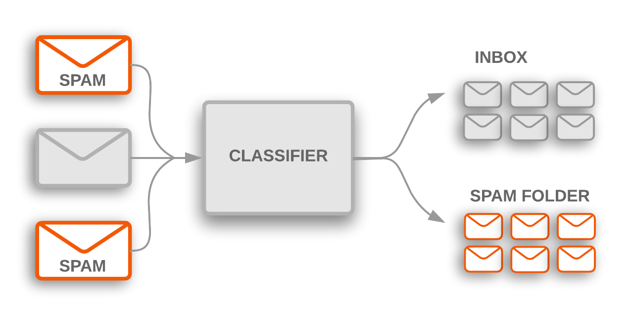
Machine Learning uses a different approach to generate a program that can make predictions from data. Instead of programming it by hand it is learned from past data. This process works if we have data instances for which we know exactly what the right prediction would have been. For example past data might be user-annotated as spam or not-spam. A machine learning algorithm can utilize such data to learn a program, a classifier, to predict the correct label of each annotated data instance.
Other successful applications of machine learning include web-search ranking (predict which web-page the user will click on based on his/her search query), placing of online advertisements (predict the expected revenue of an ad, when placed on a homepage, which is seen by a specific user), visual object recognition (predict which object is in an image - e.g. a camera mounted on a self-driving car), face-detection (predict if an image patch contains a human face or not).
The Basics
All supervised learning algorithms start with some dataset \(D = \{(\textbf{x}_1,y_1),\dots,(\textbf{x}_n,y_n)\}\), where each \(x_i\) is a d-dimensional input or feature vector, and \(y_i\) the corresponding output we call our label. We assume that these data points are drawn from some unknown distribution \(\mathcal{P}\), so
\[(\textbf{x}_i,y_i) \sim \mathcal{P}\]where we want want our \((\textbf{x}_i,y_i)\) to be independent and identically distributed (called iid).
This can be formalized by saying:
\[D = \{(\textbf{x}_1,y_1),\dots,(\textbf{x}_n,y_n)\} \subseteq \mathbb{R}^d \times \mathcal{C}\]where
- \(n\) is the size of our dataset
- \(\mathbb{R}^d\) is the d-dimensional feature space
- \(\textbf{x}_i\) is the feature vector of the \(i^{th}\) example
- \(y_i\) is the label or output of the \(i^{th}\) example
- \(\mathcal{C}\) is the space of all possible labels, or label space.
We can sum up the goal of supervised machine learning as finding a function \(h:\mathbb{R}^d \rightarrow \mathcal{C}\), such that for every new input/output pair \((\textbf{x},y)\) sampled from \(\mathcal{P}\) we have \(h(\textbf{x}) \approx y\).
Let’s see if we understand the definitions above by first looking at a few examples of feature spaces and label spaces.
Label Spaces Examples
- Binary Classification: Say we’re building a spam filter. Here we have to classes, spam and not spam. The label space is often \(\{0,1\}\) or \(\{-1,1\}\). The choice impacts how we write our loss function, but we’ll see more on that later on.
- Multi-class Classification: If we want to build an image classifier, we need to specify which classes we’re interested in (e.g. 1=horse, 2=dog, etc.). If we have \(K\) image classes, we have \(\mathcal{C}=\{1,2,\dots,K\}\).
- Regression: If we want to predict the daily temperature, we’re predicting a number which could take any value, even if some are highly improbable. In this case \(\mathcal{C} = \mathbb{R}\).
Feature Spaces Examples
- House: If we’re building a model to predict house sale prices, we might take \(\textbf{x}_i = (x_i^1,x_i^2,\dots,x_i^d)\) where \(x_i^1\) is the surface area in \(m^2\), \(x_i^2\) is the number of years ago the house was built, longitude and latitude, etc. In this case we have “hand-crafted” features, each chosen by the modeler.
- Text Document: For something like email classification, a common feature space is the so called bag-of-words. First we find all \(d\) unique words over all the documents we have. We then create the vector \(\textbf{x}_i = (x_i^1,x_i^2,\dots,x_i^d)\) for each document \(i\), where each element \(x_i^j\) tells us how often word \(j\) appears in document \(i\).
Hypothesis Classes and No Free Lunch
There are some steps we need to take on our path to finding that mysterious function $h$. A very important one is that we need to make some assumptions on what the $h$ looks like, and what space of functions we’ll be looking in. This could be linear functions, decision trees, polynomials, or whatever. These are called hypothesis spaces, usually denoted with $\mathcal{H}$. We need to make this assumption, since this choice has a big impact on how our model will generalize to new data points which aren’t present in our training data, which is the ultimate goal of machine learning.
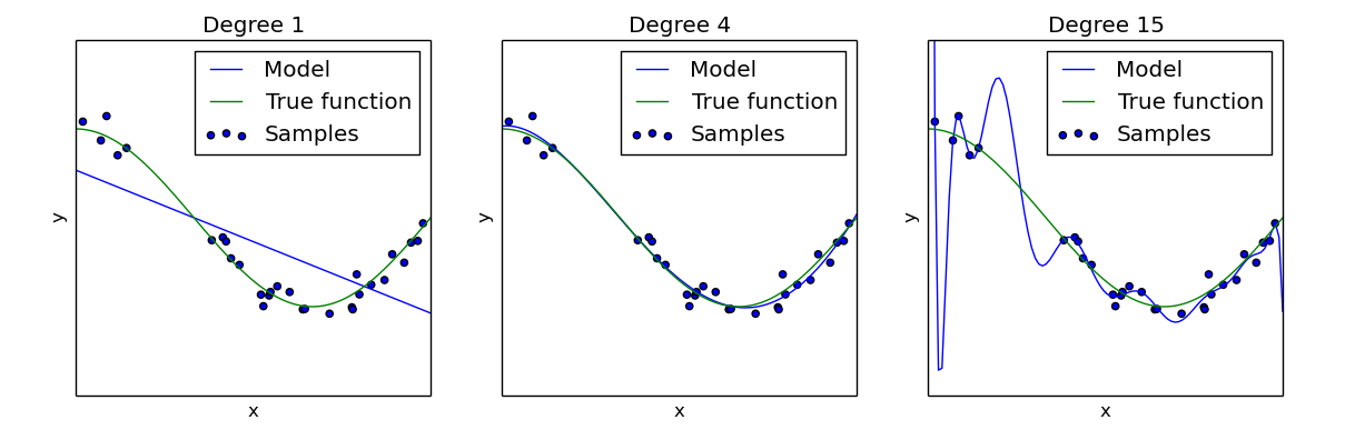
One way of understanding these hypothesis spaces is to look at how expressive they are, or how flexible they are in capturing the structure of a dataset. One of the challenges of machine learning is finding the right balance of flexibility, where not enough causes underfitting or bias, and too much causes overfitting or variance. One way of describing this expressiveness is the Vapnik–Chervonenkis dimension.
Each machine learning algorithm makes assumptions which restrict its search to a specific space of functions. There’s no way around this due to the No Free Lunch Theorem, which you could summarize as “there’s no ultimate ML algorithm which is the best on all problems”.
Loss Functions
After having been given a dataset \(D\) and having chosen a hypothesis space \(\mathcal{H}\) of functions we can possibly learn, the next step is to find the best \(h\) in that set. The problem is, how do we define best \(h\)?
This is where a loss function \(L:\mathcal{H} \rightarrow \mathbb{R}\) comes into play, which assigns a loss to each \(h \in \mathcal{H}\). This loss number tells us how good our \(h\) is, given the data \(D\) we want it to reproduce. In general a loss function will give hypotheses \(h\) with fewer reproduction errors on \(D\) a lower loss, but there are times where you want to take additional factors into account like model complexity. We’ll return to this when we cover regularization.
With this loss function at hand, our original problem has now become an optimization problem, which is
\[\arg\min_{h \in \mathcal{H}} L(h) = \arg\min_{h \in \mathcal{H}} \frac{1}{n}\sum_{i=1}^nl(\textbf{x}_i,y|h)\]We’ll be using \(L\) for the loss of a hypothesis \(h\) given \(D\), and \(l\) for the loss of a single data pair \((\textbf{x}_i,y)\) given \(h\).
Zero-One Loss
This is one of the simplest loss functions. What this loss does is count the number of mistakes \(h\) makes for each training sample. We can state this as:
\[L(h) := \frac{1}{n}\sum_{i=1}^n\delta_{h(\textbf{x}_i)\neq y_i}\]where \(\delta\) is the Dirac delta function
\[\delta_{h(\textbf{x}_i)\neq y_i} = \begin{cases} 1 & h(\textbf{x}_i)\neq y_i \\ 0 & \text{otherwise} \\ \end{cases}\]This isn’t used much in practice since it’s non-differentiable and non-continuous, which makes it difficult to work with for optimization algorithms we be needing.
Squared Loss
This loss is generally used in regression problems where \(y_i \in \mathbb{R}\). The loss per training sample is \((h(\mathbf{x}_i) - y_i)^2\), which is the distance squared. The overall loss becomes
\[L(w):=\frac{1}{n}\sum_{i=1}^n(h(\mathbf{x}_i) - y_i)^2\]The fact that the error is squared means that large errors will be much more punishing than smaller ones, and when searching for \(h \in \mathcal{H}\) we’ll end up choosing one which would rather have lots of small errors rather than a few large ones.
Generalization
One question you might want to ask is “if we’re only looking at our data \(D\), how do we ensure our model will perform well on new data?” We’ll show why this is an important question with a little motivating example.
Given a data set \(D\), lets define a function \(h\) which just memorizes the output \(y_i\) for each input vector \(\textbf{x}_i\), or:
\[h(\textbf{x}) := \begin{cases} y_i & \text{if there exists $(\textbf{x}_i,y_i)$ such that $\textbf{x} = \textbf{x}_i$}, \\ 0 & \text{otherwise}\end{cases}\]This function would perform perfectly on our training data \(D\), but anything new which we haven’t seen before would probably be horribly wrong. So how do we ensure we don’t learn hypotheses like this?
Train Test Split
The generally used approach to avoid the above pitfall is to split our dataset \(D\) into three sets, \(D_{TR}, D_{VA}, D_{TE}\), which are usually called train, validation and test. A good split might be something like 80/10/10, although this depends on the application and size of \(D\) among other things.
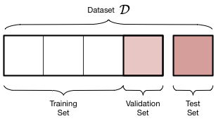
We do this at the very start of our search for \(h\). When we’re trying out all kinds of different algorithms we use the training set to search for our function \(h\), and our validation set to determine if it’s any good. Once we’ve done this numerous times and are happy with the results, we crack open the test set to see what the final accuracy is.
Train/Test Split Gone Wrong
We need to be really careful when we’re creating the split in our data. Lets take spam-filtering as an example. If we just randomly split our emails and labels into train/validation/test, create a classifier, we’d we surprised to find that our model has 0% error! Although some might think “Great, we’re done!”, it would be wiser to look into what might be happening.
After some detective work, you would discover we made a big error. Spammers create an email once and send it to millions of people. This means we have same email text in both our training set and test set. What our classifier did was just memorize which words are in those spam emails, and since the same text was in the test set it worked great.
In reality spammers change their emails frequently to avoid such classifiers, so we should be smarter too. We want our test set to mimick the settings in which our algorithm will have to function in the real world. A simple way to fix this is to split our dataset by time, so we’ll be testing on newer emails than were found in our training set.
Formalizing Generalization
We can formalize what we mean by generalization with this expression
\[\mathbb{E}_{(\textbf{x},y)\sim \mathcal{P}}\left[l(h;(\textbf{x},y))\right]\]which is the expected loss of our hypothesis, if we take the expectation over all possible input/output pairs drawn from \(\mathcal{P}\). This is really what we want to minimize, but we can’t do this directly since we don’t know what \(\mathcal{P}\) is.
This is what we’re trying to simulate with our validation set \(D_{VA}\). Since our algorithm has never seen this set, it’s as though we’re drawing that many new points from our distribution \(\mathcal{P}\)!
Summary
We defined our dataset $D$ as a set \(\{(\textbf{x}_1,y_1),\dots,(\textbf{x}_n,y_n)\}\) of data points. Given this dataset, we need to choose a hypothesis space \(\mathcal{H}\) which we will search through to find a good function \(h \in \mathcal{H}\) for which \(h(\textbf{x}) \approx y\) when \((\textbf{x},y) \sim \mathcal{P}\). We generally choose \(\mathcal{H}\) implicitly by our choice of machine learning algorithm.
Which function \(h\) is best, is decided by our choice of loss function $L$. This allows us to compare the performance of datasets on some set of data points.
In order to make sure our algorithm generalizes well after training, we split our dataset into trainging, validation and test. We training on the training set, optimize our algorithm according to the loss on the validation set, and once we’re done we use the test set to get a good approximation of how our algorithm will perform in the real world.